Research Summary for August 13, 2001
-
I have started practicing and learning GASP version 4. First
I went over a tutorial case which was the calculation of 2-D, turbulent,
transonic flow in a duct. In this case, the geometry is very similar to
the one (Sajben transonic diffuser) that we consider for our study. I made
two runs: One with a coarse grid and the other with a fine grid. These
runs gave me a general understanding of how the code works, I/O, grid sequencing
etc.
Sajben Transonic Diffuser
(STD) Case:
-
Different runs for the STD geometry were performed by using
a single zone grid with the dimensions of (81 x 51 x2). The grid file was
downloaded from the NPARC
alliance validation archive.
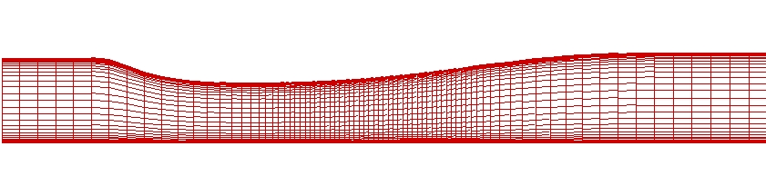
Figure 1. Single zone grid used in the transonic diffuser computation
The diffuser is 0.5583 m in length with a throat height
of 0.0439979 meters. The bottom plate of the grid is aligned in the x-axis,
with the origin located at the diffuser throat. The height of the duct
at the inlet is 1.4 throat heights, and the exit is 1.5 heights:
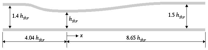
Figure 2. Geometry of the STD.
The top wall of the diffuser is defined by:
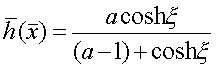 where
where
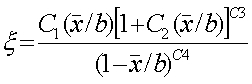 Values for the various constants are given in the table below:
Constant
|
Converging
|
Diverging
|
|
a
|
1.4114
|
1.5
|
|
b
|
-2.598
|
7.216
|
|
C1
|
0.81
|
2.25
|
|
C2
|
1.0
|
0.0
|
|
C3
|
0.5
|
-
|
|
C4
|
0.6
|
0.6
|
Boundary Conditions:
-
For the inflow boundary, a constant total pressure (P0) and
temperature were specified:
P0=134,999.1 Pa
T0=277.8 K
M0=0.46 (Inflow mach number)
-
On the upper and lower walls, the adiabatic no-slip boundary
cond. was used.
-
The outflow boundary was set to a constant static pressure
Pb (back pressure):
Pb=110,660.65 Pa for the weak shock case
Pb=97,215.50 Pa for the weak shock case
In each case, the inflow conditions were used in the computational
domain to initialize the solution.
Physical Models Used In the Computation:
-
Inviscid fluxes were calculated by using the upwind biased
3rd order accurate Roe flux scheme.
-
The Min-Mod limiter was used.
-
In the viscous fluxes, the thin-layer approximation was made
for the calculation of the viscous terms. The viscous gradients at the
solid wall were computed by using a second order, one-sided algorithm.
-
For the weak shock case, Spalart-Allmaras turbulence model
and Wilcox k-w model (1998 version) were used. For the strong shock case,
results presented here were obtained by using the Spalart-Allmaras turbulence
model.
-
As for the global iteration, Gauss-Seidel time integration
scheme was used. In each cycle, 10 Gauss Seidel inner iterations were performed
with an inner tolerance of 0.01.
-
A constant CFL number based on the freestream values were
used. The value of CFL number was set to 10. (The use of a constant CFL
number avoids oscillations in the shock position)
Results:
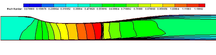
Figure 3. Mach Contours for the weak shock case. Turbulence model:
Spalart-Allmaras
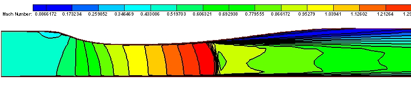
Figure 4. Mach Contours for the strong shock case. Turbulence model:
Spalart-Allmaras
-
Mean Wall Pressure Distributions:
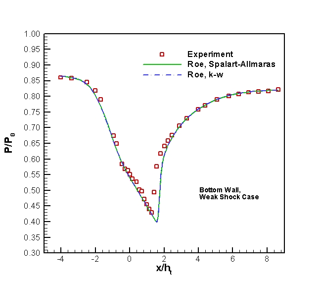
Figure 5. Mean static pressure distribution along the bottom wall of
the diffuser for the weak shock case.
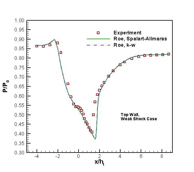
Figure 6. Mean static pressure distribution along the top wall of the
diffuser for the weak shock case.
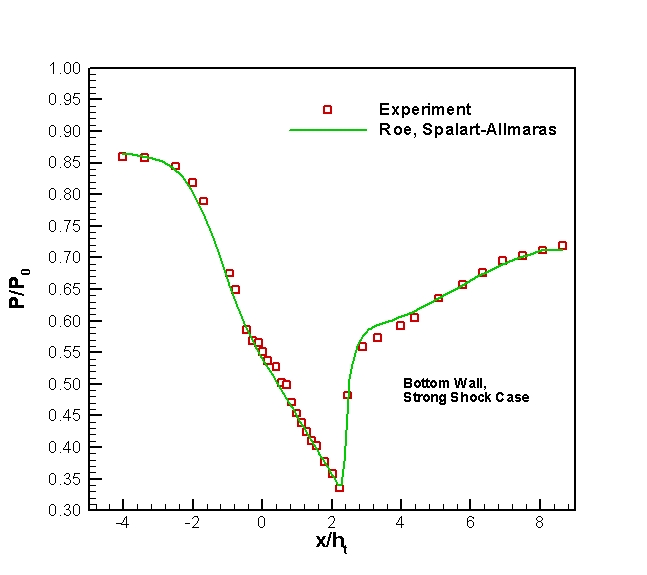
Figure 7. Mean static pressure distribution along the bottom wall of
the diffuser for the strong shock case.
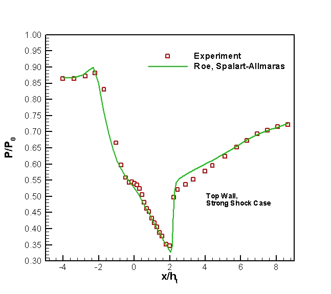
Figure 8. Mean static pressure distribution along the top wall of the
diffuser for the strong shock case.
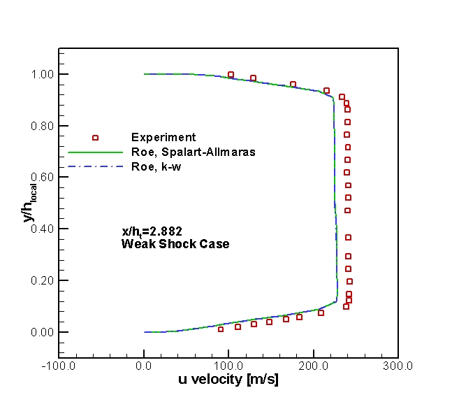
Figure 9. u velocity profiles at x/h_t=2.882 for the weak shock case
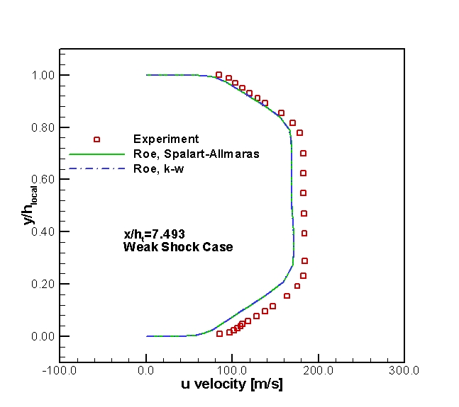
Figure 10. u velocity profiles at x/h_t=7.493 for the weak shock case
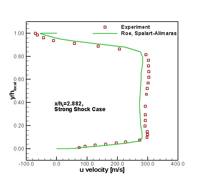
Figure 11. u velocity profiles at x/h_t=2.882 for the strong shock
case
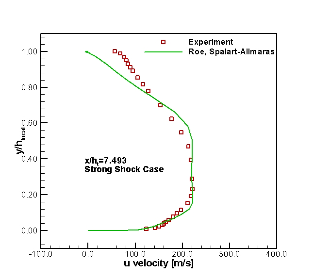
Figure 12. u velocity profiles at x/h_t=7.493 for the strong shock
case
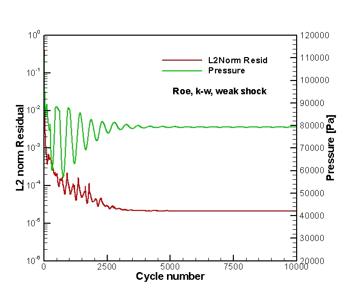
Figure 13. Convergence history of weak shock solution with Roe flux
and k-w turbulence model.
-
In the figure above, the pressure watch point was located
at i=40, j=27. This point corresponds to x/h_t=0.9375 and y/h_t=0.9678
just after the shock.